There is an inbuilt auto loan amortization schedule in Microsoft Excel accessible for free. You can use it any time by opening the ready-to-use template. Amortization Schedule is also known as a loan repayment schedule which shows the details of loan-related information.
Loan Amortization Excel 2016
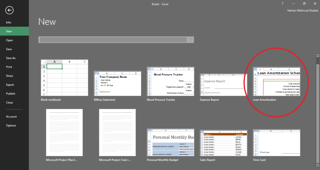
After opening the template you will be required to fill up the information in the designated fields. Then the loan amortization excel will display the results

If you want to learn how to make a loan amortization schedule using Microsoft Excel 2016 then this article is for you.
Suppose you will be required 1 Million USD for your garments machinery purchase so you are planning to take a loan from the bank. Debt is the cheapest source of finance if there is an opportunity of taking a loan then you must take it. But before taking a loan you should do a comparative study of available loan alternatives. So that you can have a better financial decisions for your business.
Bank Loan-Related Information
The loan-related information you have collected from a Bank is:
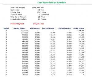
| Term Loan Amount | 1,000,000 | USD |
| Loan Period | 5 | Year |
| Interest Rate | 10% | Percent |
| Payment Terms | 1 | Times/Year |
| Total No. of Payment | 5 | Times |
| Periodic Interest Rate | 10% | Percent |
Then you need to calculate the periodic payment of your loan. To calculate this, you can use the formula and put it in your notebook and then calculate the payment.
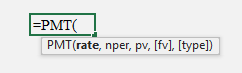
But if you use Excel then you will find an inbuilt function that will make your job easier. The function is the “PMT” function.
Calculation of Periodic payments is necessary because it will show you how much money you need to pay for each payment. This is definitely a cash outflow for you or your business. You must have to do a cash flow forecast so that you can check whether there is available money on your hand to do repayment of your loan.
Periodic Payment = $263,797 USD
- Rate = Periodic Interest Rate
- NPER = Total Number of Payment
- Pv = Present Value of the Amount that is loan amount (should input as a negative value to get the positive result)
- FV = Future Value of Loan
- Type = Payment Mechanism (Beginning of the period or ending of the period) For the beginning period payment the value is “1” (annuity due), and for the ending of the period payment the value is “0” (ordinary annuity)
Loan Amortization Schedule
| Period | Opening Balance | Total Payment | Interest Payment | Principal Payment | Closing Balance |
| 0 | 1,000,000 | – | – | – | 1,000,000 |
| 1 | 1,000,000 | 263,797 | 100,000 | 163,797 | 836,203 |
| 2 | 836,203 | 263,797 | 83,620 | 180,177 | 656,025 |
| 3 | 656,025 | 263,797 | 65,603 | 198,195 | 457,830 |
| 4 | 457,830 | 263,797 | 45,783 | 218,014 | 239,816 |
| 5 | 239,816 | 263,797 | 23,982 | 239,816 | (0) |
If are you looking for a solution to make beautiful invoices online then Luzenta would be the best solution for you.
Steps of Making Loan Amortization Schedule in Excel
- After calculating the periodic payment amount you can put the same value in all fields of the payment column.
- The zero period closing balance should be the loan amount and then the beginning balance of the first year should be the ending balance of the previous year which is zero years.
- The interest amount can be calculated by multiplying the beginning balance of that period multiplies the periodic interest rate.
- The principal amount is the difference between the payment amount in that period minus the interest amount.
- You will get the ending balance of a loan by subtracting the periodic principal amount from the beginning value of the unpaid loan amount.
- After filling in the first row you can copy the formulas to the following period then your loan repayment schedule will be there.
- At the end of the last periodic payment, your ending loan amount will be zero and this confirms that you made the loan amortization schedule successfully.
I made a simple tutorial for your better understanding, you can follow the instruction described in this video. I also added a simple template that will be convenient for your calculation.